In this post I’ll discuss a reality that is often overlooked when talking about using cloud services: Network latency matters.
Here is the test network:
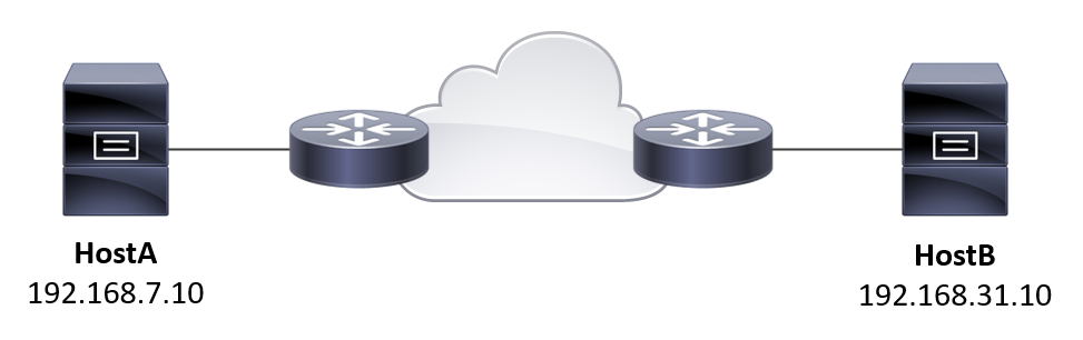
On Your Marks
Let’s first imagine that the hosts HostA and HostB are near each other, like in the same data center. The latency between the hosts is negligible:
markku@HostA:/mnt$ ping 192.168.31.10
PING 192.168.31.10 (192.168.31.10) 56(84) bytes of data.
64 bytes from 192.168.31.10: icmp_seq=1 ttl=62 time=0.475 ms
64 bytes from 192.168.31.10: icmp_seq=2 ttl=62 time=0.630 ms
64 bytes from 192.168.31.10: icmp_seq=3 ttl=62 time=0.566 ms
64 bytes from 192.168.31.10: icmp_seq=4 ttl=62 time=0.586 ms
64 bytes from 192.168.31.10: icmp_seq=5 ttl=62 time=0.624 ms
^C
--- 192.168.31.10 ping statistics ---
5 packets transmitted, 5 received, 0% packet loss, time 81ms
rtt min/avg/max/mdev = 0.475/0.576/0.630/0.057 ms
markku@HostA:/mnt$
That’s about 0.6 ms latency (or RTT, round-trip time, or RTD, round-trip delay) between the hosts.
For demonstration, I have created a Samba file share on HostB, and mounted that on /mnt on HostA. We can see the files there over the network:
markku@HostA:/mnt$ ls -lv
total 102400
-rwxr-xr-x 1 root root 10485760 May 2 20:18 test1
-rwxr-xr-x 1 root root 10485760 May 2 20:19 test2
-rwxr-xr-x 1 root root 10485760 May 2 20:19 test3
-rwxr-xr-x 1 root root 10485760 May 2 20:19 test4
-rwxr-xr-x 1 root root 10485760 May 2 20:19 test5
-rwxr-xr-x 1 root root 10485760 May 2 20:19 test6
-rwxr-xr-x 1 root root 10485760 May 2 20:19 test7
-rwxr-xr-x 1 root root 10485760 May 2 20:19 test8
-rwxr-xr-x 1 root root 10485760 May 2 20:19 test9
-rwxr-xr-x 1 root root 10485760 May 2 20:19 test10
markku@HostA:/mnt$ du -sh
100M .
markku@HostA:/mnt$
So there is 100MB of data in the file share. Let’s get the files over to HostA (and send them to /dev/null right away as we don’t need to consider any disk write latencies here):
markku@HostA:/mnt$ time cat test* > /dev/null
real 0m0.959s
user 0m0.000s
sys 0m0.042s
markku@HostA:/mnt$ time cat test* > /dev/null
real 0m0.961s
user 0m0.000s
sys 0m0.042s
markku@HostA:/mnt$ time cat test* > /dev/null
real 0m0.950s
user 0m0.005s
sys 0m0.036s
markku@HostA:/mnt$
The results are quite uniform, it takes just under a second to transfer 100 MB of data. As effective transfer speed, that means just over 880 Mbps (100*1024*1024 B = 839 Mb, in 0.95 s). For the record, this test setup has 1 Gbps network interfaces, so the observed transfer speed matches well with that (as there are protocol overheads involved as well).
Off You Go
Now, let’s move HostA to the favorite cloud platform, because that’s what you are supposed to do nowadays, right? In this setup we do the “move” by adding some delay in the network (in this test network we adjusted the network emulation settings in the VyOS routers):
markku@HostA:/mnt$ ping 192.168.31.10
PING 192.168.31.10 (192.168.31.10) 56(84) bytes of data.
64 bytes from 192.168.31.10: icmp_seq=1 ttl=62 time=40.6 ms
64 bytes from 192.168.31.10: icmp_seq=2 ttl=62 time=40.7 ms
64 bytes from 192.168.31.10: icmp_seq=3 ttl=62 time=40.7 ms
64 bytes from 192.168.31.10: icmp_seq=4 ttl=62 time=40.7 ms
64 bytes from 192.168.31.10: icmp_seq=5 ttl=62 time=40.7 ms
^C
--- 192.168.31.10 ping statistics ---
5 packets transmitted, 5 received, 0% packet loss, time 12ms
rtt min/avg/max/mdev = 40.586/40.669/40.717/0.136 ms
markku@HostA:/mnt$
Now there is about 40 ms latency between the hosts. In Europe that’s like half the continent in distance in practice, or from Finland to Central Europe (and back).
Let’s do the same file transfers again:
markku@HostA:/mnt$ time cat test* > /dev/null
real 0m7.277s
user 0m0.003s
sys 0m0.050s
markku@HostA:/mnt$ time cat test* > /dev/null
real 0m7.363s
user 0m0.000s
sys 0m0.051s
markku@HostA:/mnt$ time cat test* > /dev/null
real 0m7.045s
user 0m0.000s
sys 0m0.043s
markku@HostA:/mnt$
What happened? We have the same hosts, same data, and the same 1 Gbps network between the hosts, but the transfer time was increased from under 1 second to over 7 seconds. That means an effective transfer speed of under 120 Mbps, in a gigabit network!
The effect of latency in the network for the applications really depend on the applications’ use of the network. For chatty applications that send lots of packets back and forth the effect is huge, but for bulk transfer applications, when tuned for latency, the effect is maybe not that much.
In our test case we had a file share implemented with Samba, and the protocol used for transferring the data was SMB2 (Server Message Block 2), so this is roughly the same situation as Windows workstations accessing Windows servers’ file shares. The SMB protocols are known to suffer from high latency.
Think about implementing new virtual desktop infrastructure (VDI) in a public cloud somewhere, and using your on-premises Active Directory with the VDI instances. When the user logs in or uses some specific applications, there is high possibility that the VDI instance needs to download some data from a file share in your own data center, and that can take some time if there is high latency between the cloud and on-premises systems.
Basically, whenever one end of the connection needs to wait for something from the other end before it can proceed, high latency causes issues, regardless of the available bandwidth of the connection. Imagine sending instant messages to your friend in the nearby village, but not with your phone but with pigeons (like in RFC1149). The end result is not so quick chat. The same happens with networking over long distances: it takes a (relatively) long time to get responses, and it all adds up to the total time.
TCP (Transmission Control Protocol) is very often used as the transport protocol over the IP (Internet Protocol) networks. TCP needs the receiver to acknowledge all the data the sender has sent, which means that by nature the latency affects it. By clever use of TCP buffers and TCP window scaling the sender can send more data while acknowledgements are still on their way, and thus the transfer can happen efficiently even over high-latency network. This of course only helps with applications and protocols that move big chunks of data without requiring application-specific acknowledgements all the time. For applications that require instant responses to queries (like applications connecting to databases while querying lots of different things) this doesn’t help.
Some applications can fight the latency by using multiple parallel transport streams. While single streams still suffer the effects of delay, the combined throughput will be higher than with one stream only.
What Can You Do?
You need to architect the application system internals so that there are no high-latency connections between the parts that require lots of communication with fast responses. Think about application server and database server placements in the same cloud provider, and maybe even in the same availability zone.
You also need to consider the externals of the application systems: Where are the users connecting the system from, and with which kind of protocols and expectations? Which other systems this application systems will communicate with, and with which kind of protocols and expectations? Don’t place your application in a data center far away from other parties if the application cannot deal with the high latency.
Commonly applications are developed and tested in closed environments where all the parts of the system are near each other. Then, when building the system for production from ground up, the circumstances can be very different. Be sure to test your application in realistic implementations right from the beginning. That way you know how your application behaves in real situations, and you can better fight the effects of latency in your application.
If using ready-made application components there can be settings available specifically for handling high latency, for example configuring concurrent connections for transferring data. As circumstances vary, be sure to study and test any such settings carefully before changing them in production implementations.
Recently I had to transfer lots of multi-gigabyte files to an Amazon S3 bucket using AWS CLI. Even though the data connection had several gigabits of bandwidth available, I was only able to achieve about 100 Mbps for the transfer speed. When rechecking the configuration settings for AWS CLI S3 commands I realized that the default for
max_concurrent_requestsis 10. That’s the setting that makes it possible to achieve better throughput in high latency situations. I set it to 1 instead, and the transfers were now able to achieve speed of 300 Mbps! The background of the situation is that the files were located on an USB-connected and USB-powered external 2.5″ spinning hard drive, and apparently the device couldn’t keep up with many simultaneous I/O requests all over the disk. So, what works for some, doesn’t perhaps work for others, so you need to know your environment.
There is also a whole category of networking equipment that is specialized in accelerating networking protocols over high-latency networks. These wide area network (WAN) accelerators or optimizers usually act as middle boxes in both ends of the network connections (as either physical or virtual appliances, or as a feature on an existing firewall or other networking device), and they can optimize specific protocols on the fly so that the effects of latency can be minimized. For some protocols the benefits are huge, and that can be real life-saver for businesses that depend on geographically distant sites communicating with each other with otherwise unoptimized protocols. Implementing WAN optimization requires careful planning and implementation as it is not a one-size-fits-all solution for WAN networking problems.